Number one again!

I was pleased to see that my SQL Expert book is yet again listed as a number one best seller this afternoon by Amazon.com’s book ranking system for two of the book’s categories:

  • Computers and Technology -> Databases and Big Data -> Oracle
  • Computers and Technology -> Certification -> Oracle

Trailing are excellent books in their own right, including many authored or co-authored by Oracle ACE Directors: a brand new Oracle Public Cloud book co-authored by Charles Kim, Mark Rittman‘s Business Intelligence book from Oracle Press, and Steve Feuerstein‘s legendary PL/SQL book.

I’m busy working on a new book from Oracle Press, more on that in the very near future – stay tuned! In the meantime, the 047 book makes a great holiday present for anyone in your life who wants to become a certified SQL Expert!

Below is the screenshot from the “Databases and Big Data” category:

Oracle SQL Expert Number One on the Amazon Best Selling Charts 11/29/2016 for its category.

Larry Ellison, and “cloud computing” vs. “utility computing”

“Everyone doesn’t have their own well at their house … we tap into the water network, we tap into the electricity network … we get better service at a lower price by having our water come from a utility … we’ll experience the same economic advantages … as we get our data from an information utility.” – Larry Ellison, Oracle Open World, September 18, 2016, spoken during his keynote presentation: “The Cloud: A New Era of Utility Computing”

Don’t be misled.   Larry Ellison is not late to the Cloud Party.  Consider this quote from 1998:

… Larry Ellison, the founder and CEO of the Oracle Corporation, has frequently mused at what life would be like if common household appliances had the same complexity of maintenance as a PC … “Sorry, I can’t go out tonight, I’m staying home so I can upgrade my TV to version 7.0.” … Ellison’s argument … the PC must become as easy to use as any common household appliance.

In a recent presentation … Ellison was asked … if the network will be stable enough—won’t it crash from time to time? … Ellison’s response … what is the last thing that crashed on you: your telephone, or Windows … ? The audience roared with laughter, making the answer obvious …

The number of networks we already depend on is impressive: plumbing, electricity, highways, television, radio—all networks professionally run by others … Why should a computer user experience anything different?

— Excerpted from Chapter 27, “Oracle Web Application Server”, in the book “Oracle8 Server Unleashed” published by Macmillan Computer Publishing.

That’s a brilliant quote, isn’t it?  You better say ‘yes’ because I selected that 1998 quote for my chapter in that “Oracle8 Server Unleashed” book. (I only authored that one chapter, this work was the result of a few dozen authors, I only authored the one chapter.)

I selected that quote because of Larry Ellison’s leadership.  Ellison, way ahead of his time, had already seen the potential of the World Wide Web and its underlying protocol, HTTP, all of which had been invented barely five years prior.  Ellison had already seen the vision and was leading the charge towards “utility computing”.

So I was thrilled to see Ellison keeping that phrase alive yesterday at OOW.  To me, “utility” computing is significantly more descriptive than the phrase “cloud” computing.  Clouds paint images of vague, nebulous, fragmented things somewhere far away, without specificity or form or shape.  But utility computing is much more descriptive of what is really intended: a ubiquitous workhorse that is simultaneously both specific and dependable, scientifically complex at it core, cutting edge in its usefulness, yet easy for everyone to access and use for common purposes.

Cloud computing is not just a “computer somewhere else”, as I’ve heard it described – that’s a funny one-liner and I’ve been guilty of laughing at it myself.  But cloud computing – utility computing – is significantly much more than that.  It is a series of complex hardware, network, and software components, brought together in an easy-to-configure, easy-to-access, ever-present simple interface through which an end-user can quickly set up (provision) whatever resources he or she needs quickly to meet whatever business requirement is currently demanding attention, in a more cost-effective manner than ever before, by compartmentalizing the various desired components and optimizing their deployment.

It is true that Amazon Web Services has much of the market momentum at the moment, and has captured a lot of the headlines in the tech industry.

But the truth is that Oracle is still, to this moment, the unquestioned leader in all forms of serious professional business software applications, and he has been actively and purposely working for years to leverage the power of the network in support of business objectives.  The multi-year re architecture of most of the world’s leading enterprise resource planning (ERP) applications is just one example of what they’ve done toward this goal.

This week’s Oracle Open World should be very eventful.

For Larry Ellison’s keynote last night, see this link, but recognize this link might not survive much longer than OOW 2016: https://www.oracle.com/openworld/on-demand/index.html

For an OOW YouTube channel highlight that might survive the link above, see here: https://youtu.be/S1p_TcS9bxk


Rio Mid-Games: Gold Medals Per Capita So Far

Four years ago I blogged about the fact that medal counts are often reported on a per-country basis without regard for the population of any country. I’ve always thought that approach to be silly. The per-capita medal count is much more interesting to me.

So this morning I used Bing to get the latest count by country of gold medals at the ongoing Rio Olympics.  I included only those nations that have won two or more gold medals.

I then visited Wikipedia to get recent population counts for those nations.

I used all this data to determine the per-capita win per nation and ranked them.  The results are below.

Ranking Country Per Capita Ratio
(Descending Order)
Gold Medal Count Population Date Population Reported
1 Jamaica 7.34418E-07 2 2,723,246 31-Dec-14
2 New Zealand 6.37423E-07 3 4,706,450 16-Aug-16
3 Hungary 6.10811E-07 6 9,823,000 1-Jan-16
4 Croatia 4.77251E-07 2 4,190,669 31-Dec-15
5 Netherlands 3.52389E-07 6 17,026,640 16-Aug-16
6 Australia 2.48343E-07 6 24,160,100 16-Aug-16
7 United Kingdom 2.45738E-07 16 65,110,000 30-Jun-15
8 Switzerland 2.39762E-07 2 8,341,600 31-Mar-16
9 Greece 1.84196E-07 2 10,858,018 1-Jan-15
10 Cuba 1.77952E-07 2 11,239,004 31-Dec-15
11 Belgium 1.76637E-07 2 11,322,674 1-Jun-16
12 Italy 1.31871E-07 8 60,665,551 1-Jan-16
13 South Korea 1.18107E-07 6 50,801,405 1-Jul-16
14 Kazakhstan 1.12656E-07 2 17,753,200 1-May-16
15 Germany 1.10064E-07 9 81,770,900 30-Sep-15
16 France 1.04891E-07 7 66,736,000 1-Jul-16
17 Spain 8.61356E-08 4 46,438,422 1-Jan-16
18 United States 8.01855E-08 26 324,248,000 16-Aug-16
19 North Korea 7.91108E-08 2 25,281,000 1-Jul-16
20 Russia 7.50345E-08 11 146,599,183 1-May-16
21 Uzbekistan 6.33406E-08 2 31,575,300 1-Jan-16
22 Canada 5.53166E-08 2 36,155,487 1-Apr-16
23 Japan 5.51225E-08 7 126,990,000 1-Jul-16
24 Poland 5.20329E-08 2 38,437,239 31-Dec-15
25 Kenya 4.52934E-08 2 44,156,577 1-Jul-15
26 Colombia 4.09887E-08 2 48,793,900 16-Aug-16
27 Thailand 3.04279E-08 2 65,729,098 31-Dec-15
28 Iran 2.51689E-08 2 79,463,100 16-Aug-16
29 China 1.08836E-08 15 1,378,220,000 16-Aug-16
30 Brazil 9.68457E-09 2 206,514,000 16-Aug-16

You could argue that some country populations and/or medal counts are too small to prove anything other than an interesting anomaly.  Or not.  But there’s no question that Hungary and the Netherlands are very impressive, each with six gold medals for an overall per-capita rate that’s dramatically higher than, for example, Great Britain, the United States, and especially China, who – in spite of their very high medal count, is actually very far behind the other nations on a per capita basis.

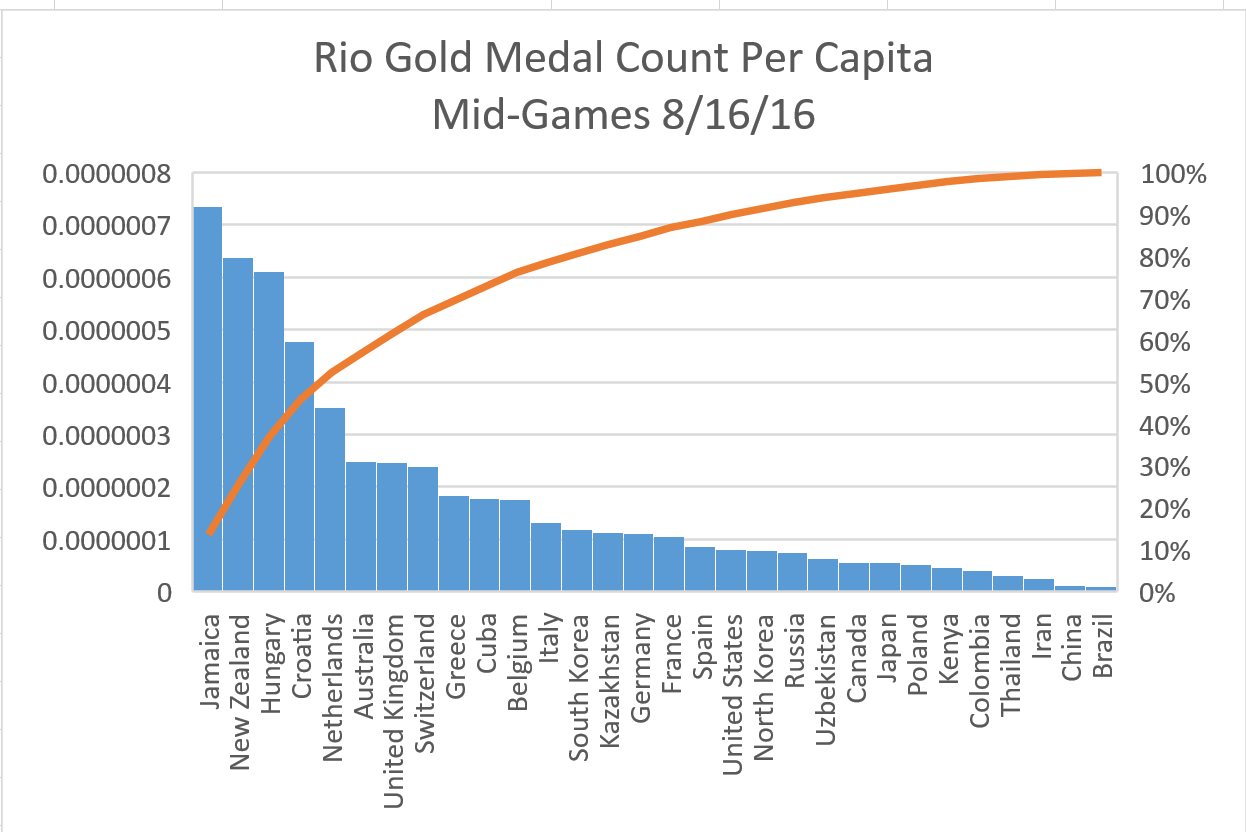
These are the results presented graphically, which I created using Microsoft Excel, captured with the built-in “snipping” tool in Microsoft Windows: :

The Pareto Line seems to curve most significantly above Hungary and the Netherlands, which have the most striking performance in terms of size of population and count of gold medals.  Also – note how far back China ranks.  They might have a lot of medals, but they also have the largest population in the world.

To me, this sort of analysis is much more interesting than the simple medal count that doesn’t account for population.


Sources:

  • Gold Medal Count as of 8/16/2016: http://www.bing.com/search?pc=COSP&ptag=D073116-A855B9C56E1&form=CONBDF&conlogo=CT3335450&q=gold+medal+count+by+country
  • Country Population Data: https://en.wikipedia.org/wiki/List_of_countries_and_dependencies_by_population

Amazon Web Services (AWS) – System Log

Here’s an easy way to review the system log of an EC2 Instance using Amazon Web Service (AWS):

  • Navigate to the Management Console (the starting point of everything in AWS)
  • Click “EC2”
  • Click “Running Instances”
  • Choose the instance you’re interested in by clicking the empty square to its right and turning it solid blue
  • Click Actions -> Instance Settings -> Get System Log

See below for what your screen should look like.

The result will be a pop-up window displaying the system log:

That’s it!

MySQL Migration: from Drupal to WordPress

I just migrated this Skere9 blog from a Drupal implementation at SiteGround to a WordPress instance at Amazon Web Services.  I’ve been a customer of AWS for three years and finally decided to move this blog to the same platform where I’ve been doing other work.  It’s cost-effective and AWS provides significantly greater control over numerous aspects of the deployment.

Note:  I have one author – myself – and I did not migrate any comments with this move.  I will add those later.

The Drupal version is 7.4.1.  The WordPress version is 4.5.3.

To migrate the blog posts, I took the following steps.

  • I temporarily installed phpMyAdmin at the Drupal site to export the “node” and “field_data_body” tables from Drupal.  (Note: this could have also been done using MySQL directly.)
  • I installed phpMyAdmin at the WordPress site to import the Drupal tables.  (Note: this could have also been done using MySQL directly.) I edited the phpMyAdmin config file to restrict access to phpMyAdmin to my own IP address.
  • I executed the script below via phpMyAdmin at the WordPress site to pull data from the imported Drupal tables and insert that data into the WordPress database.
INSERT INTO wp_posts
(       id
      , post_author
      , post_date
      , post_date_gmt
      , post_content
      , post_title
      , post_status
      , comment_status
      , ping_status
      , post_name
      , post_modified
      , post_modified_gmt
      , post_parent
      , guid
      , menu_order
      , post_type
)
SELECT
        a.nid+100
      , 1
      , FROM_UNIXTIME(a.created)
      , FROM_UNIXTIME(a.created)
      , b.body_value
      , a.title
      , 'publish'
      , 'open'
      , 'open'
      , CONCAT('dr-', a.nid+100)
      , FROM_UNIXTIME(a.changed)
      , FROM_UNIXTIME(a.changed)
      , 0
      , CONCAT('http://skere9.com/?p=', a.nid+100)
      , 0
      , 'post'
FROM     node a LEFT JOIN (field_data_body b)
            ON (a.nid = b.entity_id)
WHERE    type = 'blog'
ORDER BY a.nid

A few important notes about the above code:

  • I had fewer than 100 existing posts in the WordPress instance- it was a brand new installation.  This is why I only added 100 to the ID, to create unique identifiers.
  • I transformed the data formats from UNIX to plain text, as required by the source and target tables.
  • I chose to enter each value into the WordPress “postname” field with a “dr-” prefix – for “Drupal”.  But of course that could have been anything, or nothing at all – no prefix is required here.
  • The “_gmt” fields in the target database are being treated by my WordPress implementation as the same as the local time.  Presumably GMT refers to Greenwich Mean Time, comparable to UTC.  I’m in the USA eastern time zone (New York City zone – I’m in Washington, DC), so presumably the offset should be 5 hours but the existing WordPress implementation I have isn’t treating the times differently.  Therefore I didn’t treat them differently either – I made the “created” timestamp the same for the local and GMT entry, and did the same for the “changed” timestamp.

It all worked like a charm.

GROUP BY on a GROUP BY

Here’s something I’ve been working on lately – a number of metrics across large data sets where I want to determine aggregates of aggregates.  I can’t present the actual data I’m working with here, but this is an illustrative example.  Consider the data set below.

SQL> SELECT   *
  2  FROM     shop_orders;

        ID CATEGORY   ITEM_N
---------- ---------- --------------------
         1 Office     Stapler
         2 Fruit      Banana
         3 Bread      French Bread
         4 Steak      Ribeye
         5 Fish       Bass
         6 Crackers   Saltines
         7 Fish       Swordfish
         8 Fruit      Pear
         9 Bread      Rolls
        10 Crackers   Chips
        11 Steak      Prime Rib
        12 Bakery     Birthday Cake
        13 Fish       Salmon
        14 Fish       Flounder
        15 Cleaners   Detergent
        16 Bakery     Donuts
        17 Office     Ink Cartridges
        18 Steak      Filet Mignon
        19 Vegetable  Broccoli
        20 Steak      Flank
        21 Fruit      Raspberry
        22 Sundries   Shampoo
        23 Steak      Salisbury
        24 Vegetable  Radish
        25 Vegetable  Mushroom
        26 Pharmacy   Band-aids
        27 Pharmacy   Aspirin
        28 Sundries   Toothbrush
        29 Sundries   Shampoo
        30 Cereal     Bran
        31 Cereal     Corn Flakes
        32 Cleaners   Soap
        33 Cereal     Oatmeal

33 rows selected.

One glance at the data and you can see the category values repeat. But how often do they repeat? Which categories recur the most frequently? What if you needed to determine which categories have the greatest number of values, and which don’t?

To determine this, we can start with a GROUP BY, like this.

SQL> SELECT   category, COUNT(*) CT
  2  FROM     shop_orders
  3  GROUP BY category;

CATEGORY       CT
---------- ----------
Cereal              3
Fruit               3
Crackers            2
Vegetable           3
Office              2
Steak               5
Pharmacy            2
Fish                4
Bread               2
Cleaners            2
Sundries            3
Bakery              2

12 rows selected.

Now let’s move the GROUP BY to an inline view, and do a GROUP on the GROUP BY, like this.

SQL> SELECT COUNT(b.category) ct_category, b.ct ct_item_n
  2  FROM
  3    ( SELECT   a.category, COUNT(a.item_n) CT
  4  	 FROM	  shop_orders a
  5  	 GROUP BY a.category
  6    ) b
  7  GROUP BY b.ct
  8  ORDER BY b.ct DESC;

CT_CATEGORY  CT_ITEM_N
----------- ----------
          1          5
          1          4
          4          3
          6          2

Voila – there is one category that recurs five times, one recurs 4 times, four recur three times, and finally six categories have two values each.

In a relatively small data set like this, the answers might be obvious. I’ve been working with very large rows that number in the tens of millions and queries like this have been invaluable in confirming data shape and patterns.

If you wish to experiment with these SQL statements, here is the code to create the sample table and sample data.

DROP   TABLE shop_orders;
CREATE TABLE shop_orders
(   id       NUMBER
  , category VARCHAR2(15)
  , item_n   VARCHAR2(20)
);
INSERT INTO shop_orders VALUES ( 1, 'Office', 'Stapler');
INSERT INTO shop_orders VALUES ( 2, 'Fruit', 'Banana');
INSERT INTO shop_orders VALUES ( 3, 'Bread', 'French Bread');
INSERT INTO shop_orders VALUES ( 4, 'Steak', 'Ribeye');
INSERT INTO shop_orders VALUES ( 5, 'Fish',  'Bass');
INSERT INTO shop_orders VALUES ( 6, 'Crackers', 'Saltines');
INSERT INTO shop_orders VALUES ( 7, 'Fish', 'Swordfish');
INSERT INTO shop_orders VALUES ( 8, 'Fruit', 'Pear');
INSERT INTO shop_orders VALUES ( 9, 'Bread', 'Rolls');
INSERT INTO shop_orders VALUES (10, 'Crackers', 'Chips');
INSERT INTO shop_orders VALUES (11, 'Steak', 'Prime Rib');
INSERT INTO shop_orders VALUES (12, 'Bakery', 'Birthday Cake');
INSERT INTO shop_orders VALUES (13, 'Fish', 'Salmon');
INSERT INTO shop_orders VALUES (14, 'Fish', 'Flounder');
INSERT INTO shop_orders VALUES (15, 'Cleaners', 'Detergent');
INSERT INTO shop_orders VALUES (16, 'Bakery', 'Donuts');
INSERT INTO shop_orders VALUES (17, 'Office', 'Ink Cartridges');
INSERT INTO shop_orders VALUES (18, 'Steak', 'Filet Mignon');
INSERT INTO shop_orders VALUES (19, 'Vegetable', 'Broccoli');
INSERT INTO shop_orders VALUES (20, 'Steak', 'Flank');
INSERT INTO shop_orders VALUES (21, 'Fruit', 'Raspberry');
INSERT INTO shop_orders VALUES (22, 'Sundries', 'Shampoo');
INSERT INTO shop_orders VALUES (23, 'Steak', 'Salisbury');
INSERT INTO shop_orders VALUES (24, 'Vegetable', 'Radish');
INSERT INTO shop_orders VALUES (25, 'Vegetable', 'Mushroom');
INSERT INTO shop_orders VALUES (26, 'Pharmacy', 'Band-aids');
INSERT INTO shop_orders VALUES (27, 'Pharmacy', 'Aspirin');
INSERT INTO shop_orders VALUES (28, 'Sundries', 'Toothbrush');
INSERT INTO shop_orders VALUES (29, 'Sundries', 'Shampoo');
INSERT INTO shop_orders VALUES (30, 'Cereal', 'Bran');
INSERT INTO shop_orders VALUES (31, 'Cereal', 'Corn Flakes');
INSERT INTO shop_orders VALUES (32, 'Cleaners', 'Soap');
INSERT INTO shop_orders VALUES (33, 'Cereal', 'Oatmeal');

COMMIT;

There you go! Have fun!

Generating Test Data

Here’s a quick way to generate dummy data for performing tests that require lots of records.

SQL> DROP   TABLE lots_o_data;

Table dropped.

SQL> CREATE TABLE lots_o_data
  2  (	 id	  NUMBER
  3    , name	  VARCHAR2(5)
  4    , category VARCHAR2(26)
  5  );

Table created.

SQL> INSERT INTO lots_o_data VALUES (1, 'Lotso', 'Wow this is a lot of data.');

1 row created.

SQL> INSERT INTO lots_o_data VALUES (2, 'More',  'Bunches and bunches.');

1 row created.

SQL> COMMIT;

Commit complete.

SQL> INSERT INTO lots_o_data
  2  	 SELECT a.id, a.name, b.category
  3  	 FROM lots_o_data a CROSS JOIN lots_o_data b;

4 rows created.

SQL> COMMIT;

Commit complete.

SQL> INSERT INTO lots_o_data
  2  	 SELECT a.id, a.name, b.category
  3  	 FROM lots_o_data a CROSS JOIN lots_o_data b;

36 rows created.

SQL> COMMIT;

Commit complete.

SQL> INSERT INTO lots_o_data
  2  	 SELECT a.id, a.name, b.category
  3  	 FROM lots_o_data a CROSS JOIN lots_o_data b;

1764 rows created.

SQL> COMMIT;

Commit complete.

SQL> INSERT INTO lots_o_data
  2  	 SELECT a.id, a.name, b.category
  3  	 FROM lots_o_data a CROSS JOIN lots_o_data b;

3261636 rows created.

SQL> COMMIT;

Commit complete.

SQL> SELECT COUNT(*)
  2  FROM   lots_o_data;
  COUNT(*)                                                               ----------                                                             3263442                                                                      
SQL> SPOOL OFF

Note the following

  • With only four INSERT … SELECT statements based on a Cartesian product, we were able to generate over 3 million rows of data.
  • A few more INSERT … SELECT statements could easily result in billions of rows of data.

If you need a lot of data for performance testing or capacity testing, this is an easy way to get however much you require.

I have been working on building a data lake environment in anticipation of a series of large data feeds I’m expecting soon and found this to be a useful approach to preparing the environment.

“What Child Is This” – Martina McBride and Michael W. Smith

From the 2015 Country Music Association (CMA) Country Music Awards show, featuring Martina McBride and Michael W. Smith.

Merry Christmas everyone!

Updated 12/26/2021: I updated the link to replace the original that had gone dead – it was here: https://www.youtube.com/embed/GKvMq1N59HQ.